Backlinks
1 Escape Velocity and Gravitational Potential Energy
1.1 Newton's Universal Gravitation Law
where, \(\vec{F_g}\) is the force of gravity on \(M_2\); \(M_1\) and \(M_2\) are two point masses; \(G\) the universal gravitation constant; \(r\) the magnitude of the vector \(\vec{r}\) from \(M_1\) to \(M_2\) and \(\hat{r}\) the unit vector in the \(\vec{r}\) direction.
1.2 Equation for Gravitational Potential Energy
1.2.1 Needed Definitions
To begin, we need to modify the Newton's Universal Gravitation Law to fit the parameters of the scenario. Namely, we need to treat both Earth and our object as point masses, and assign \(M_1\) to be Earth and \(M_2\) to be our object.
Also, it is necessary to define the coordinate system: that our object, \(M_2\), is defined to be to the left/more negative side of the coordinate compared to the location occupied by the Earth, \(M_e=M_1\) (as, per the problem, the "zero" point is set at \(r = \infty\).)
We could therefore claim \(\vec{r}\) as a vector of the displacement pointing from the object to the Earth; it is, therefore, positive as it points from the zero point (\(r=\infty\)) to the Earth.
Hence, with the necessary variable substitutions as highlighted before, we arrive at the following equation:
\begin{equation} \vec{F_{em}}(r) = \frac{-GM_eM_2}{r^2} \end{equation}1.2.2 Deducing Gravitational Potential energy
The general equation for work from \(A\to B\) is defined as follows:
\begin{equation} W(A \to B) = \int^B_A \vec{F(x)} d\vec{r} \end{equation}In this case, as we will be deducing the total gravitational potential energy as per the setup above, we need to be integrating upon \(\vec{F_{em}}(r) dr\). We know that the direction of gravitation is in the direction of \(-{\hat{r}}\). Hence, the integral is therefore:
\begin{equation} W(A \to B) = \int^B_A {\frac{-GM_eM_2}{r^2} dr\hat{r}\hat{r}} = \int^B_A {\frac{-GM_eM_2}{r^2} dr} \end{equation}Determining the total gravitation potential energy will therefore involve evaluating the integral:
\begin{eqnarray} W(A \to B) &=& \int^B_A{\frac{-GM_eM_2}{r^2} dr} \\ W(A \to B) &=& -GM_eM_2 \int^B_A{\frac{1}{r^2} dr} \\ W(A \to B) &=& -GM_eM_2 \int^B_A{r^{-2} dr} \\ W(A \to B) &=& \frac{GM_eM_2}{r} |^B_A \end{eqnarray}To figure the constant of integration, we take the fact that \(W(A\to B)=-\Delta PE(A\to B)\) due to the conservation of potential energy.
We set the begging of experiment as \(A = \infty\), tracking its attraction to point \(B\).
\begin{equation} W(\infty \to B) &=& \frac{-GM_eM_2}{B} \end{equation}Therefore:
\begin{equation} PE_B - PE_A = \frac{-GM_eM_2}{B} \end{equation}As we set the beginning of the experiment to be the point at \(A=\infty\), \(PE_A = 0\). Furthermore, as distance to \(B\) is the entirety of travel, \(r=B\).
Therefore:
\begin{equation} -\Delta PE = \frac{GM_eM_2}{r} \end{equation}1.3 Escape Velocity
To deduct the escape velocity of the Earth, our object \(M_2\) must do enough work such that the work Earth exerts upon it — as deducted above — is canceled out.
1.3.1 Calculation Setup
Hence, to figure the escape velocity, we must deduct the kinetic energy needed to perform the exact work deducted above in the opposite direction by substituting the statement of change in kinetic energy and \(-\Delta PE\) as derived above. That,
\begin{equation} \Delta KE = -\Delta PE \Rightarrow \frac{1}{2}M_2 v = \frac{GM_eM_2}{r} \end{equation}Also, as the object to escape Earth's gravitation is starting at the surface of Earth, \(r = R_e\), the radius of the earth.
1.3.2 Deducing Escape Velocity
The final calculations after substitution is therefore simply a matter of isolating \(v\), the magnitude velocity.
\begin{align} \frac{1}{2}M_2 v^2 &= \frac{M_eM_2}{R_e} \\ v^2 &= 2\frac{GM_e}{R_e} \\ v &= \sqrt{2\frac{GM_e}{R_e}} \end{align}1.3.3 Calculating Escape Velocity
Taking \(G = 6.674 \times 10^{-11} m^3 \frac{m^3}{kg\ s^2}\), \(M_e = 5.97 \times 10^{24} kg\), and \(R_e = 6.371 \times 10^6 km\)…
\begin{equation} v \approx 1.119 \times 10^4 \frac{m}{s} = 2.503 \times 10^4 \frac{M}{h} \end{equation}2 Center of Mass
2.1 Finding an Expression for the Position of the Center of Mass
The net force of a system is described as:
\begin{equation} \sum^n_{i=1} \vec{F_{net,i}} = (\sum^n_{i=1} m_i) \ddot{\vec{r_{CM}}} \end{equation}where, \(\vec{F_{net,i}}\) is the net force on \(m_i\), \(\vec{r_{CM}}\) the position vector of the center of mass \(CM\).
In order to isolate \(\vec{r_{CM}}\), the equation above must be integrated twice w.r.t. time, namely:
\begin{equation} \int \sum^n_{i=1} \vec{F_{net,i}} dt = \int (\sum^n_{i=1} m_i) \ddot{\vec{r_{CM}}} dt \end{equation}with the integrals performed twice.
For this evaluation, we will also set \(\sum^n_{i=1} m_i = M\), define \(\vec{a_i}\) as acceleration of \(m_i\), \(\vec{r_i}\) as position of \(m_i\), and apply Newton's second law:
We first perform the first integration:
\begin{align} \int \sum^n_{i=1} \vec{F_{net,i}} dt &= \int (\sum^n_{i=1} m_i) \ddot{\vec{r_{CM}}} dt \\ \sum^n_{i=1} m_i \int \vec{a_i} dt &= M \int \ddot{\vec{r_{CM}}} dt \\ \sum^n_{i=1} m_i \int \frac{d^2\vec{r_i}}{dt^2} dt &= M \int \frac{d^2\vec{r_{CM}}}{dt^2} dt \\ \sum^n_{i=1} m_i \frac{d\vec{r_i}}{dt} &= M \frac{d\vec{r_{CM}}}{dt} + C_1 \\ \end{align}Given the statement for velocity, we need to integrate again to figure position.
\begin{align} \int (\sum^n_{i=1} m_i \frac{d\vec{r_i}}{dt}) dt &= \int M \frac{d\vec{r_{CM}}}{dt} + C_1 dt \\ \sum^n_{i=1} m_i \int \frac{d\vec{r_i}}{dt} dt &= M \int \frac{d\vec{r_{CM}}}{dt} + C_1 dt \\ \sum^n_{i=1} m_i \vec{r_i} + C_2 &= M \vec{r_{CM}} \\ \frac{1}{M} \sum^n_{i=1} m_i \vec{r_i} + C_2 &= \vec{r_{CM}} \end{align}In the case of the first integral application, the constant of integration — \(C_1\) — is defined to be zero due to the fact that, were it to be nonzero, the center of mass would be traveling at a faster rate than that of the object. As the object increases in speed, the center of mass would therefore increase in speed as well more than the object: leading it to travel away from the object, which would be absurd.
In the latter case, the constant of integration — \(C_2\) — is equally defined as zero due to the fact that, were the value to be nonzero, the center of mass would perhaps be consistently ahead or behind from the object, which would equally be absurd.
Collecting all constants, as both constants of integration is defined to be at zero, we could set \(C=0\). As such, the position \(\vec{r_{CM}}\) of the center of mass \(CM\) is therefore:
\begin{equation} \vec{r_{CM}} = \frac{1}{M} \sum^n_{i=1} m_i \vec{r_i} \end{equation}Where, \(M\) is the total mass of the system, \(m_i\) the mass of component \(i\) of the system, and \(\vec{r_i}\) the position of \(m_i\).
Center of mass can also be defined for a more general system, as follows:
\begin{equation} \vec{r_{CM}} = \frac{\int y dm}{\int dm} \end{equation}that, the center of mass is the position at which the differential mass-weighted sum is the same.
2.2 Simplifying to ignore internal forces
Because of Newton's Third Law, if forces acted internal to a system, the target of the force — given its inside the system — will preform an equal and opposite reaction. Hence, the net internal force will be \(0\), meaning that we could ignore internal forces.
Because of the fact that \(\vec{r_{CM}} = \frac{1}{M} \sum^n_{i=1} m_i \vec{r_i}\) as derived above, \(\vec{r_{CM}}\) changes when the system as a whole moves. However, internal forces does not do this, meaning the existence of internal forces does not change \(\vec{r_{CM}}\).
This fact allows for a simplification of the equation:
\begin{equation} \sum^n_{i=1} \vec{F_{net,i}} = (\sum^n_{i=1} m_i) \ddot{\vec{r_{CM}}} \end{equation}to:
\begin{equation} \sum^m_{j=1} \vec{F_{ext,j}} = M \ddot{\vec{r_{CM}}} \end{equation}by applying \(\sum^n_{i=1} m_i = M\) as per aforementioned and the external forces argument above.
3 Calculating the Center of Mass
For an system with the following points, calculate its center of mass:
| Component Vector | Mass |
|---|---|
| (1,-4,1) | 1kg |
| (-3,-2,6) | 2kg |
| (2,5,-3) | 3kg |
| (-2,4,6) | 4kg |
Applying the expression for the center of mass above, we deduct that the center of mass of this object is located at point \(\frac{\{(1-3\times 2 + 2 \times 3 - 2 \times 4), (-4-2\times 2 + 5 \times 3 + 4 \times 4), \(1+6\times 2 -3 \times 3 + 6 \times 4)\}}{1+2+3+4} = (-0.7, 2.3, 2.8)\).
This center of mass is then plotted visually in an interactive GeoGebra graph. A render of which is shown below:
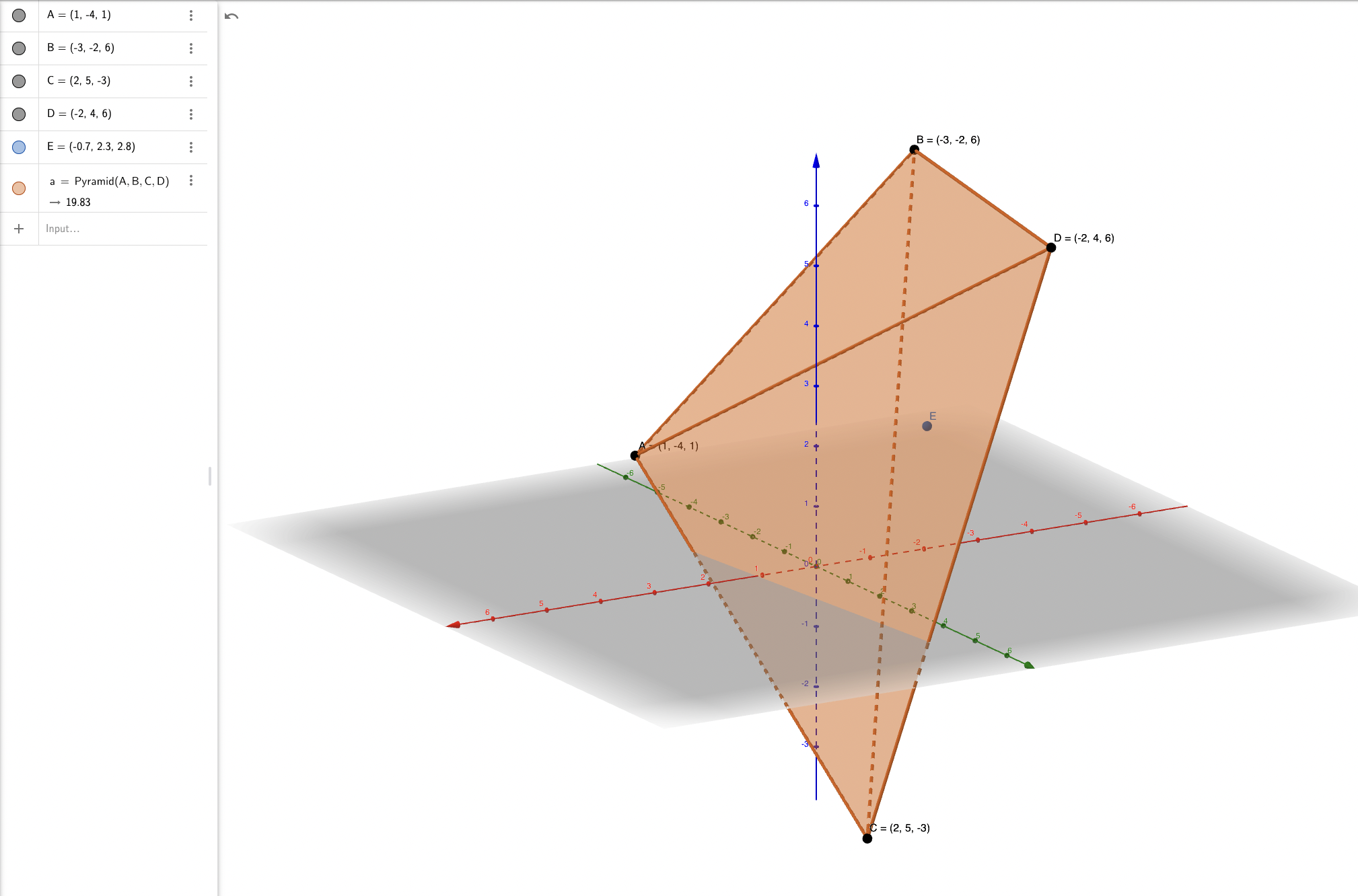
As one could see, the center of mass is in the center of the object, but shifted towards \(D\) as it is the "heaviest" point in the system.