Backlinks
1 Setup
The ball launcher problem involves an energetic optimization to figure, given the situation as shown in the above image, the parameters \(h_0\) and \(\theta_0\) that would best create a maximum launch distance \(x_f\).
In this problem, we will define the axis such that the "lower-left" corner of the wood block (corner sharing \(x\) value of the starting position of the marble, but on the "ground") as \((-w,0)\), where \(w\) is the width of the wooden block. Therefore, we derive the x-value of the location of the launch of the projectile as \(x=0\). We define the direction towards with the marble is launching as positive-x, so as the marble rolls, its position's \(x\) value increases. We will define the location of the marble before starting as positive \(y\), and as the marble decreases in height, its position's \(y\) value decreases.
We define the start of the experiment as time \(t_0\), the moment the marble leaves the track and travels as a projectile as \(t_1\), and the end — in the moment when the marble hits the ground — as \(t_f\). We will call the marble \(m_0\).
2 Figuring the Velocity at \(t_1\)
In order to expedite the process of derivation, we will leverage an energetic argument instead of that of kinematics for figuring the velocity at launch. The change-in-height that \(m_0\) experiences before \(t_1\) is \(\Delta h = H-h_0\). Therefore, the potential energy expenditure is \(\Delta PE_{grav} = mg\Delta h = m_0 g (H - h_0)\). Assuming that the marble starts out with 0 kinetic energy, we deduct that, at the moment of it finishing its descent, it will possess kinetic energy \(KE = 0+m_0 g (H - h_0) = m_0 g (H - h_0)\).
For this derivation, for now, we ignore \(KE_{rotational}\), hence, we could roughly deduct the statement that \(KE_{translational} \approx m_0 g (H - h_0)\).
Creating this statement, we could deduct a statement that we could leverage to solve for the velocity at \(t_1\) named \(\vec{v_0}\).
\begin{align} m_0g(H-h_0) =& \frac{1}{2}m_0\vec{v_0}^2 \\ g(H-h_0) =& \frac{1}{2}\vec{v_0}^2 \\ 2g(H-h_0) =& \vec{v_0}^2 \\ \vec{v_0} =& \sqrt{2g(H-h_0)} \end{align}This velocity vector could be easily split into its two constituent parts. Namely:
\begin{cases} \vec{v_0_x} = \sqrt{2g(H-h_0)}cos(\theta_0)\\ \vec{v_0_y} = \sqrt{2g(H-h_0)}sin(\theta_0)\\ \end{cases}3 Figuring the Maximum Possible Travel Distance
Here, we devise an function for \(x_f\) w.r.t. \(\vec{v_0_y}\), \(\vec{v_0_x}\), \(h_0\), \(m_0\).
3.1 Setup for Kinematics
We first will leverage the parametric equations for position in kinematics in order to ultimately result in a function for \(x_f\).
\begin{cases} x(t) = \frac{1}{2}a_0_xt^2 + v_0_xt + x_0 \\ y(t) = \frac{1}{2}a_0_yt^2 + v_0_yt + y_0 \\ \end{cases}Given the situation of our problem, we could modify the pair as follows:
\begin{cases} x(t) = v_0_xt \\ y(t) = \frac{-1}{2}gt^2 + v_0_yt + h_0 \\ \end{cases}as,
- there are no acceleration in the x-direction at the point of launch
- the only acceleration in the y-direction is that due to gravity
- the start x-position of the marble at launch is, as defined above, \(x=0\)
- the start y-position of the marble at launch is, as defined above, \(y=h_0\)
3.2 Setup for Solution
We first create a set of equations modeling the location of the marble at \(t_f\).
\begin{cases} x(t_f) = x_f = v_0_xt_f = t_f\sqrt{2g(H-h_0)}cos(\theta_0)\\ y(t_f) = 0 = \frac{-1}{2}g{t_f}^2 + v_0_y t_f + h_0 = \frac{-1}{2}g{t_f}^2 + t_f\sqrt{2g(H-h_0)}sin(\theta_0) + h_0 \end{cases}We first solve for \(t_f\), and supply it to the first equation.
\begin{equation} t_f = \frac{x_f}{\sqrt{2g(H-h_0)}cos(\theta_0)} \end{equation}Finally, we substitute the definition of \(t_f\) into \(y(t_f)\).
\begin{equation} y(t_f) = 0 = \frac{-1}{2}g{\frac{x_f}{\sqrt{2g(H-h_0)}cos(\theta_0)}}^2 + {\frac{x_f}{\sqrt{2g(H-h_0)}cos(\theta_0)}}\sqrt{2g(H-h_0)}sin(\theta_0) + h_0 \end{equation}We will now proceed to simplify the expression further
\begin{align} 0 =& \frac{-1}{4} \frac{{x_f}^2}{(H-h_0) cos^2(\theta_0)} + x_f tan(\theta_0) + h_0 \\ =& \frac{-1}{4} \frac{{x_f}^2}{(H-h_0)}cos^{-2}(\theta_0) + x_f tan(\theta_0) + h_0 \\ =& \frac{-1}{4} \frac{1}{(H-h_0)}{x_f}^2cos^{-2}(\theta_0) + x_f tan(\theta_0) + h_0 \end{align}3.3 Solution at \(\theta_0 = 0\)
We begin by first solving for the expression for \({x_f}^2\) at \(\theta_0 = 0\).
\begin{align} 0 =& \frac{-1}{4} \frac{1}{(H-h_0)}{x_f}^2cos^{-2}(\theta_0) + x_f tan(\theta_0) + h_0 \\ 0 =& \frac{-1}{4} \frac{1}{(H-h_0)}{x_f}^2 + h_0 \\ -h_0 =& \frac{-1}{4} \frac{1}{(H-h_0)}{x_f}^2\\ 4h_0 =& \frac{1}{(H-h_0)}{x_f}^2\\ {x_f}^2 =& 4h_0(H-H_0) \end{align}3.3.1 Finding \(\frac{d{x_f}^2}{dh_0}\)
Remember, given the setup of the problem, \(x_f\) is optimized when \({x_f}^2\) is optimized. This is due to the fact that \(x_f\) could not be negative, and it is representing a maximum travel distance. Hence, we will optimized \({x_f}^2\) for ease of calculation.
\begin{align} {x_f}^2 =& 4h_0(H-H_0) \\ \frac{d{x_f}^2}{dh_0} =& \frac{d}{dh_0} 4h_0(H-h_0) \\ =& 4\frac{d}{dh_0} h_0(H-h_0) \\ =& 4 ((H-h_0) - h_0) \\ =& 4H-4h_0 - 4h_0 \\ =& 4H-8h_0 \end{align}3.3.2 Optimizing \(\frac{d{x_f}^2}{dh_0}\)
The optimization of this statement is fairly simple. We set \(\frac{d{x_f}^2}{dh_0}=0\), and solve for \(h_0\).
\begin{align} {x_f}^2 =& 4H-8h_0 \\ \Rightarrow 0 =& 4H-8h_0 \\ \Rightarrow 8h_0 =& 4H \\ \Rightarrow h_0 =& \frac{1}{2}H \end{align}Hence, the most optimal height at which to launch the marble launcher, given a horizontal launch, is half of the initial height.
3.4 Solution at arbitrary \(\theta_0\)
3.4.1 Solving and optimizing for \(\frac{dx_f}{d\theta_0}\)
We need to maximize \(\frac{dx_f}{d\theta_0}\) as one out of two components to optimize for. Once we figure that value, we then supply the corresponding maximum value then optimize again for \(\frac{h_0}{d\theta_0}\). The position equations above could be leveraged to figure a value for \(x_f\).
- Finding \(\frac{dx_f}{d\theta_0}\)
We leverage implicit differentiation to figure a value for \(\frac{dx_f}{d\theta_0}\). We set \(x_f\) as a differentiable function, and \(h_0\) and \(H\) as both constants.
\begin{align} 0 =& \frac{-1}{4} \frac{1}{(H-h_0)}{x_f}^2cos^{-2}(\theta_0) + x_f tan(\theta_0) + h_0 \\ \Rightarrow \frac{d}{d\theta_0} 0 =& \frac{d}{d\theta_0} (\frac{-1}{4} \frac{1}{(H-h_0)}{x_f}^2cos^{-2}(\theta_0) + x_f tan(\theta_0) + h_0) \\ \Rightarrow 0 =& \frac{-1}{4} \frac{1}{(H-h_0)}\frac{d}{d\theta_0} {x_f}^2cos^{-2}(\theta_0) + \frac{d}{d\theta_0} x_f tan(\theta_0) + \frac{d}{d\theta_0} h_0 \\ \Rightarrow 0 =& \frac{-1}{4} \frac{1}{(H-h_0)} ((\frac{d}{d\theta_0} {x_f}^2) cos^{-2}(\theta_0) + {x_f}^2 (\frac{d}{d\theta_0} cos^{-2}(\theta_0))) + \\& ((\frac{d}{d\theta_0} x_f) tan(\theta_0) + (\frac{d}{d\theta_0} tan(\theta_0)) x_f) + 0 \\ \Rightarrow 0 =& \frac{-1}{4(H-h_0)} ((2{x_f} \frac{dx_f}{d\theta_0}) cos^{-2}(\theta_0) + {x_f}^2 (2cos^{-3}(\theta_0) sin(\theta_0))) + \\& (\frac{dx_f}{d\theta_0} tan(\theta_0) + sec^2(\theta_0) x_f)\\ \Rightarrow 0 =& \frac{-1}{4(H-h_0)} (2{x_f} \frac{dx_f}{d\theta_0}) cos^{-2}(\theta_0) + \frac{-1}{4(H-h_0)} {x_f}^2 (2cos^{-3}(\theta_0) sin(\theta_0)) + \\& \frac{dx_f}{d\theta_0} tan(\theta_0) + sec^2(\theta_0) x_f\\ \Rightarrow & \frac{1}{4(H-h_0)} {x_f}^2 (2cos^{-3}(\theta_0) sin(\theta_0)) - sec^2(\theta_0) x_f \\& = \frac{-1}{4(H-h_0)} (2{x_f} \frac{dx_f}{d\theta_0}) cos^{-2}(\theta_0) + \frac{dx_f}{d\theta_0} tan(\theta_0)\\ \Rightarrow & \frac{1}{4(H-h_0)} {x_f}^2 (2cos^{-3}(\theta_0) sin(\theta_0)) - sec^2(\theta_0) x_f \\& = \frac{dx_f}{d\theta_0} \frac{-1}{2(H-h_0)} {x_f} cos^{-2}(\theta_0) + \frac{dx_f}{d\theta_0} tan(\theta_0)\\ \Rightarrow & \frac{1}{4(H-h_0)} {x_f}^2 (2cos^{-3}(\theta_0) sin(\theta_0)) - sec^2(\theta_0) x_f \\& = \frac{dx_f}{d\theta_0} (\frac{-1}{2(H-h_0)} {x_f} cos^{-2}(\theta_0) + tan(\theta_0))\\ \Rightarrow & \frac{dx_f}{d\theta_0} = \frac{\frac{(cos^{-3}(\theta_0) sin(\theta_0))}{2(H-h_0)} {x_f}^2 - sec^2(\theta_0) x_f }{(\frac{-1}{2(H-h_0)} {x_f} cos^{-2}(\theta_0) + tan(\theta_0))} \end{align} - Optimizing for \(x_f\) for \(\theta_0\) via \(\frac{dx_f}{d\theta_0}\)
We now set \(\frac{dx_f}{d\theta_0}=0\) in order to figure critical points for the value of \(x_f\).
\begin{align}f \frac{dx_f}{d\theta_0} =& \frac{\frac{(cos^{-3}(\theta_0) sin(\theta_0))}{2(H-h_0)} {x_f}^2 - sec^2(\theta_0) x_f }{(\frac{-1}{2(H-h_0)} {x_f} cos^{-2}(\theta_0) + tan(\theta_0))} \\ \Rightarrow 0 =& \frac{\frac{(cos^{-3}(\theta_0) sin(\theta_0))}{2(H-h_0)} {x_f}^2 - sec^2(\theta_0) x_f }{(\frac{-1}{2(H-h_0)} {x_f} cos^{-2}(\theta_0) + tan(\theta_0))} \\ \Rightarrow 0 =& \frac{(cos^{-3}(\theta_0) sin(\theta_0))}{2(H-h_0)} {x_f}^2 - sec^2(\theta_0) x_f \\ \Rightarrow sec^2(\theta_0) x_f =& \frac{(cos^{-3}(\theta_0) sin(\theta_0))}{2(H-h_0)} {x_f}^2 \\ \Rightarrow sec^2(\theta_0) =& \frac{(cos^{-3}(\theta_0) sin(\theta_0))}{2(H-h_0)} x_f \\ \Rightarrow 2sec^2(\theta_0)(H-h_0) =& (cos^{-3}(\theta_0) sin(\theta_0)) x_f \\ \Rightarrow \frac{2(H-h_0)}{x_f} =& \frac{(cos^{-3}(\theta_0) sin(\theta_0))}{sec^2(\theta_0)} \\ \Rightarrow \frac{2(H-h_0)}{x_f} =& \frac{sin(\theta_0)}{cos^3(\theta_0) sec^2(\theta_0)} \\ \Rightarrow \frac{2(H-h_0)}{x_f} =& \frac{sin(\theta_0)}{cos(\theta_0)} \\ \Rightarrow \frac{2(H-h_0)}{x_f} =& tan(\theta_0) \\ \Rightarrow \theta_0 =& arctan(\frac{2(H-h_0)}{x_f}) \end{align}As there is one critical point per the range, and that there must be at least one maximum point, we determine that the derived expression will maximize \(x_f\) for a given solved \(x_f\). To figure the actual statement that would optimize for both,
3.4.2 Solving and optimizing for \(x_f\)
We will now return to our original expression for the final y-position (\(=0\)) to create an expression for \(x_f\).
- Solving for \(x_f\)
We first take the previous expression for \(x_f\) and supply the expression for \(\theta_0\).
\begin{align} 0 =& \frac{-1}{4} \frac{1}{(H-h_0)}{x_f}^2cos^{-2}(\theta_0) + x_f tan(\theta_0) + h_0 \\ 0 =& \frac{-1}{4} \frac{1}{(H-h_0)}{x_f}^2sec^{2}(arctan(\frac{2(H-h_0)}{x_f})) + x_f tan(arctan(\frac{2(H-h_0)}{x_f})) + h_0 \\ 0 =& \frac{-1}{4} \frac{1}{(H-h_0)}{x_f}^2((\frac{2(H-h_0)}{x_f})^2 +1) + x_f (\frac{2(H-h_0)}{x_f}) + h_0 \\ 0 =& \frac{-1}{4} \frac{1}{(H-h_0)} ((2(H-h_0))^2 + {x_f}^2) + 2(H-h_0) + h_0 \\ 0 =& \frac{-1}{4} ((4(H-h_0)) + \frac{{x_f}^2}{(H-h_0)}) + 2(H-h_0) + h_0 \\ 0 =& (-(H-h_0) - \frac{{x_f}^2}{4(H-h_0)}) + 2(H-h_0) + h_0 \\ \frac{{x_f}^2}{4(H-h_0)} =& -(H-h_0) + 2(H-h_0) + h_0 \\ {x_f}^2 =& -4(H-h_0)(H-h_0) + {4(H-h_0)}2(H-h_0) + {4(H-h_0)}h_0 \\ {x_f}^2 =& -4(H-h_0)^2 + 8(H-h_0)^2 + 4h_0(H-h_0) \\ {x_f}^2 =& 4(H-h_0)^2 + 4h_0(H-h_0) \\ \end{align} - Finding \(\frac{d{x_f}^2}{dh_0}\)
We know that, by optimizing for \({x_f}^2\), \(x_f\) is optimized due to the setup of the problem of the behavior of the length of line.
Hence, we take the first derivative, though of \({x_f}^2\) w.r.t. \(h_0\) and with \(H\) held constant.
\begin{align} {x_f}^2 =& 4(H-h_0)^2 + 4h_0(H-h_0) \\ \Rightarrow \frac{d{x_f}^2}{d h_0} =& \frac{d}{d h_0} (4(H-h_0)^2 + 4h_0(H-h_0)) \\ =& 4\frac{d}{d h_0} (H-h_0)^2 + 4\frac{d}{d h_0} h_0(H-h_0) \\ =& 4\frac{d}{d h_0} (H-h_0)^2 + 4((H-h_0) \frac{d}{d h_0} h_0 + h_0 \frac{d}{d h_0} (H-h_0) ) \\ =& 4\frac{d}{d h_0} (H-h_0)^2 + 4((H-h_0) - h_0) \\ =& -8(H-h_0) + 4(H-h_0) - 4h_0\\ =& -4(H-h_0) - 4h_0\\ =& -4H + 4h_0 - 4h_0\\ =& -4H \end{align} - Optimizing for \(x_f\)
The optimization of \(x_f\) requires a little bit more thinking of the scenario of the problem. \(H\) must be a positive number, and the expression for \({x_f}^2\) appears to be a straight line with slope \(-4H\).
Given \(H>0\), \(-4H<0\), and the slope of \({x_f}^2\) is negative — as \(h_0\) increases, \({x_f}^2\) decreases. Given \(h_0\) must be positive, then, \(h_0_{optim} = 0\).
3.4.3 Solving for the Actual Optimum of \(\theta_0\)
We return to following statement:
\begin{equation} \theta_0 =& arctan(\frac{2(H-h_0)}{x_f}) \end{equation}The expression we derived above for \(x_f\) under optimal conditions is, per the previous statement:
\begin{align} {x_f}^2 =& 4(H-h_0)^2 + 4h_0(H-h_0) \\ \Rightarrow {x_f} =& \sqrt{4(H-h_0)^2 + 4h_0(H-h_0)} \end{align}And substituting the statement for \(x_f\) back into the expression above, in addition to the optimal value \(h_0 = 0\) derived earlier, we derive that
\begin{align} \theta_0 =& arctan(\frac{2(H-h_0)}{x_f}) \\ \Rightarrow \theta_0 =& arctan(\frac{2(H-h_0)}{\sqrt{4(H-h_0)^2 + 4h_0(H-h_0)}}) \\ =& arctan(\frac{2(H)}{\sqrt{4(H)^2}}) \\ =& arctan(1) \\ =& 45^{\circ} \end{align}And hence, given an arbitrary angle and an arbitrary height to launch, the most optimal scenario is to make the launch point fully on the floor at an \(45^{\circ}\) angle from the plane of the floor.
4 Additional Figures
4.1 Projected Range w.r.t. varying \(h_0\) at optimal \(\theta_0\)
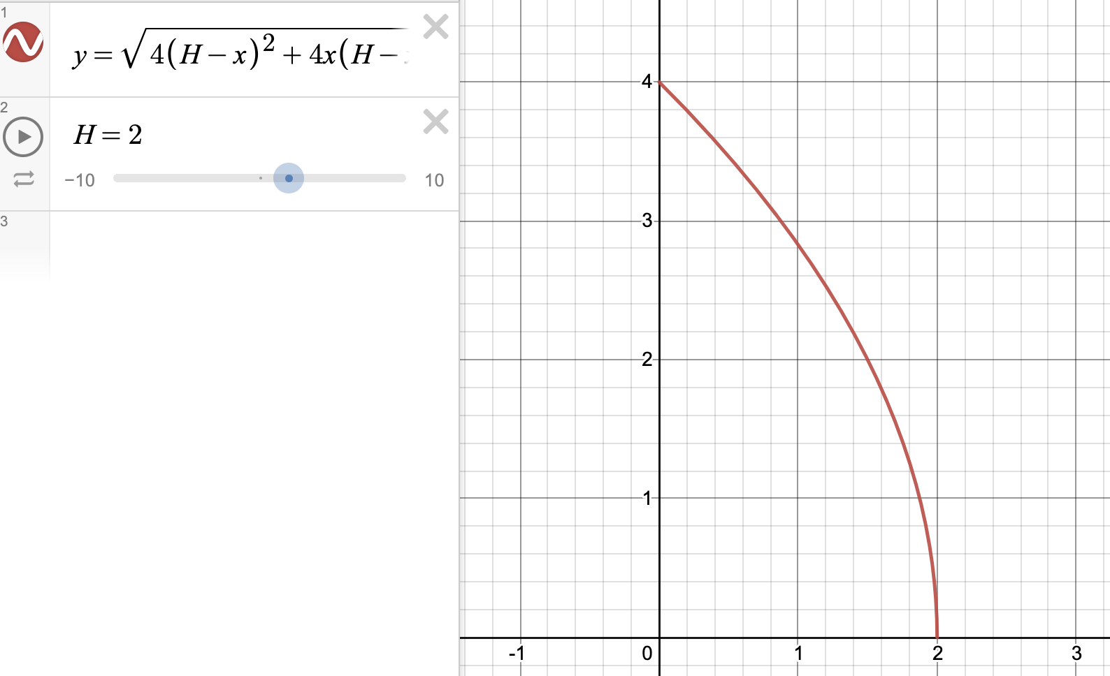
This figure is rendered in an Interactive Desmos Plot, the initial launch height, \(H\), is fixed at an arbitrary non-zero value of \(2\).
4.2 Projected Range w.r.t. varying \(h_0\) at \(\theta_0 = 0\)
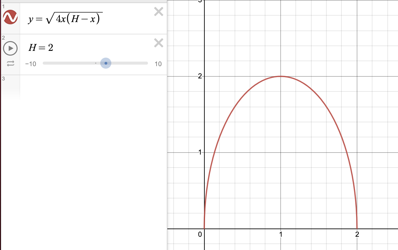
This figure is rendered in another Interactive Desmos Plot, the initial launch height, \(H\), is again fixed at an arbitrary non-zero value of \(2\).
As one could see, a parabolic relationship could be seen such that the most optimal value is at exactly \(\frac{1}{2}H\).