Backlinks
1 Setup
library(tidyverse)
library(TSA)
2 Data Sourcing
We first grab the data.
dataset_raw <- read.csv("./09162021_3rd_fl_jar_small_bead.csv")
dataset_tibble <- tibble(dataset_raw
#+begin_quote
#+end_quote
)

# rename tibble titles
dataset_tibble <- dataset_tibble %>% rename(time = Time..sec., max_height_x=Max.Height.X, max_height_y=Max.Height.Y)
3 Basic plotting
3.1 Time vs. Max Height
Plot time against max height.
g <- dataset_tibble %>% ggplot()
g <- g + geom_line(aes(x=time, y=max_height_y))
g
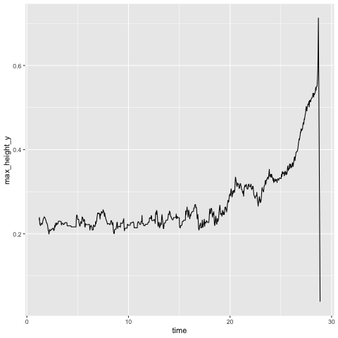
We should probably chop off the end bit, because that's just the chain flinging itself off.
dataset_sliced <- dataset_tibble %>% slice_head(n=which(dataset_tibble$max_height_y == max(dataset_tibble$max_height_y)))
And plotting again…
g <- dataset_sliced %>% ggplot()
g <- g + geom_line(aes(x=time, y=max_height_y))
g
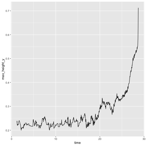
We will do the same thing
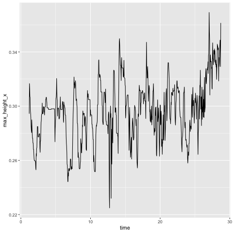
3.2 Time vs. X-Value at Max Height
We will plot and slice the same bit too, but for the x-value.
g <- dataset_sliced %>% ggplot()
g <- g + geom_line(aes(x=time, y=max_height_x))
g
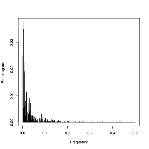
The wave could be ran through an fft.
dataset_sliced$max_height_x %>% periodogram()
There's more, but I will write that up later.