Backlinks
1 Tiling the Pringlehouse
As a review, our pringles shaped house has the following parametres:
\begin{equation} \begin{cases} x(t) = 30cos(t)\\ y(t) = 20sin(t)\\ \end{cases} \end{equation}and the roof is defined by:
\begin{equation} r(x,y) = \frac{1}{400}\left(\sqrt{3}x-y\right)^2 - \frac{1}{400}\left(\sqrt{3}y-x\right)^2 + 10 \end{equation}We will first convert the above function into rectangular bounds to take the area of.
\begin{align} &x = 30cos(t) \\ \Rightarrow &\frac{x}{30} = cos(t) \\ \Rightarrow &t = arccos\left(\frac{x}{30}\right) \end{align}Supplying this back to the original expression for y:
\begin{align} y &= 20sin\left(arccos\left(\frac{x}{30}\right)\right) \\ &=20\sqrt{1-\left(\frac{x}{30}\right)^2} \end{align}Therefore, the actual integral:
\begin{equation} \int_{-30}^{30} \int_{-20\sqrt{1-\left(\frac{x}{30}\right)^2}}^{20\sqrt{1-\left(\frac{x}{30}\right)^2}}\ 1 dy\ dx \end{equation}We will endeavor now to use technology.
var("x y")
f(x,y) = 1
f.integrate(y, -20*sqrt(1-(x/30)^2), 20*sqrt(1-(x/30)^2)).integrate(x, -30,30)
It appears that the area of the floor is \(600\pi\).
We can do this something for the function of the roof. We will first figure correction factor \(dA\), then take the integral as prescribed.
\begin{align} dA &= \sqrt{1+\left(\frac{\partial f}{\partial x}\right)^2+\left(\frac{\partial f}{\partial y}\right)^2} \end{align}At this point, we realize that the actual function will turn to be much too complicated to integrate by hand at this moment; therefore, we will create the expression digitally.
r(x,y) = (1/400)*(sqrt(3)*x-y)^2 - (1/400)*(sqrt(3)*y+x)^2 + 10
da = sqrt(1+r.diff(x)^2+r.diff(y)^2)
monte_carlo_integral(da.integrate(y, -20*sqrt(1-(x/30)^2), 20*sqrt(1-(x/30)^2)), [-30], [30], 10000000)
Looks like the result is converting to about \(2002.2\) for this shape.
2 Three Dimensional Region!
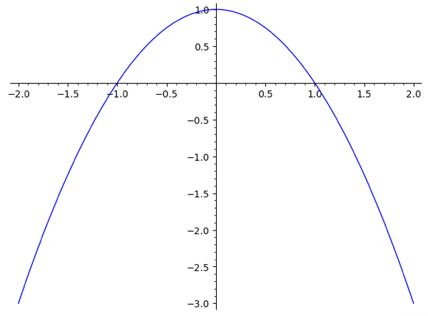
Slowly adding up the arguments to this figure reveals its general shape:
f(x) = 1-x^2
plot(f, -2, 2)
And, adding up the \(y\) component:
f(x,y) = 1-x^2-y^2
plot3d(f, (x,-2,2), (y,-2,2)) + plot3d(0, (x,-2,2), (y,-2,2))
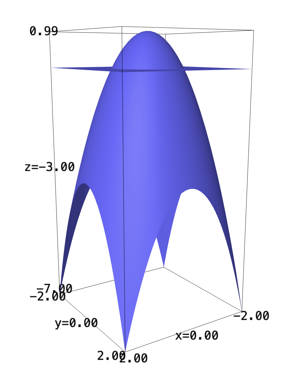
We can see that the positive component exists at \(x=[-1,1]\), \(y=[-1,1]\). If the same pattern holds, then, the maximum volume would be over areas:
\begin{equation} x=[-1,1], y=[-1,1], z=[-1,1] \end{equation}Taking the actual integral:
a(x,y,z) = 1-x^2-y^2-z^2
a.integrate(x,-1,1).integrate(y,-1,1).integrate(z,-1,1)
Shockingly, the resulting integral is \(0\). However, we can actually move the bounds to see that all other manifestations about this point would actually result in even more negative values.
a(x,y,z) = 1-x^2-y^2-z^2
a.integrate(x,-1,1).integrate(y,-1,1).integrate(z,-1,1)
Taking the Jacobian matrix of this expression would reveal that:
\begin{equation} \nabla a = \begin{bmatrix} -2x \\ -2y \\ -2z \end{bmatrix} \end{equation}We see that there is no other point but \((0,0,0)\) is the maxima, and—by the pattern of the function—holding any two variables constant and squaring the remaining one will approach \(0\) (the smallest non-negative value) at bounds \([-1,1]\). Therefore, it makes sense that the bounds prescribed would be the actual bounds desired.
3 Spinning around the origin
I suppose intuitively the function needs to be axially symmetric to actually perform this trick. This means that, for exponential functions, it has to have a square (or a square of a square, etc.) term on the \(x\) term to manifest a symmetry about \(y\) axes by the negative and positive values of \(x\) being squared the same way.
Otherwise, the "spun" result would have uneven edges that the "squishing"/dimentionality reduction of the square root will render inoperable.
Mathematically, this can be seen by the fact that \(x^2 + y^2\), when converted to polar, equals to \(r^2\). This was the only reason why we were able to actually reduce the \(x\) and \(y\) terms back down to take the square root in the first place.
Because we are manufacturing the \(y\) term from scratch, we know that the degree of both terms will be the same. Therefore, any \(x^2^n\) will be able to be reduced to $x2n+y2n = r2n$—allowing the squaring/square-root trick to take place in polar.
If, say, the power were to be odd, we no longer have this replacement and will have to be stuck in higher dimensions with a lagging \(\sin{\theta}\) or \(\cos\theta\) term—representing the fact that the non-axial-symmetry cannot be projected without loss of info to lower dimensions.