DGC 1.1 Vector Functions

\begin{equation} \vec{F} = K\frac{qq_0}{r^2}\hat{u} \end{equation}

Expanding \(K = \frac{1}{4\pi\epsilon_0}\), we arrive at

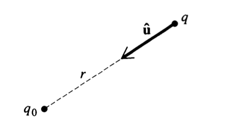
\begin{equation} \vec{F} = \frac{1}{4\pi\epsilon_0}\frac{qq_0}{r^2}\hat{u} \end{equation}

Looking at the numerator of this expression, we arrive at:

\begin{equation} qq_0 \hat{u} \end{equation}

One will realize that, if \(q,q_0\) have the same signs, they will have a positive \(qq_0\). Therefore, \(+\hat{u}\) will be pointed towards each other — meaning the charges will direct force towards themselves and hence repel; in a similar vein, if \(q,q_0\) have different signs, they will have a negative \(qq_0\), \(-\hat{u}\) will be pointed away from each other and hence the particles will push themselves towards each other.

Therefore: "like changes repel, unlike changes attract."

If there are three changes, \(q_0\), \(q_1\), \(q_2\), and \(\vec{F}_1 \Rightarrow q_1 \to q_0\), \(\vec{F}_2 \Rightarrow q_2 \to q_0\): the total net force on \(q_0\) is \(\vec{F}_1 + \vec{F}_2\).

The electrostatic field is the field that a change emits given one test change, though not counting the interaction of the test change.

\begin{equation} \vec{E}(\vec{r}) = \frac{\vec{F}(\vec{r})}{q_0} = \frac{1}{4\pi\epsilon_0}\frac{q}{r^2}\hat{u} \end{equation}

So then, if we expand this same principle to \(N\) number of test changes, though all discounting their influences:

\begin{equation} \vec{E}(\vec{r}) = \sum^N_{i=1} \frac{1}{4\pi\epsilon_0}\frac{q}{|\vec{r}-\vec{r}_i|^2}\hat{u} \end{equation}

How far away is the object from the origin at any time \(t\)

The object is, at any time \(t\), the following magnitude away from the origin:

\begin{equation} \sqrt{a^2\ cos^2(\omega\ t) + b^2\ sin^2(\omega\ t)} \end{equation}

Find the object's velocity and acceleration as functions of time

As the function is \(R^1 \to R^2\), there are no partial derivatives to be taken. Hence:

\begin{equation} \vec{r}' = \omega(-\hat{i}a\ sin(\omega\ t) + \hat{j} b\ cos(\omega\ t)) \end{equation} \begin{equation} \vec{r}'' = -\omega^2(\hat{i} a\ cos(\omega\ t) + \hat{j} b\ sin(\omega\ t)) \end{equation}

Show that the object moves on the elliptical path

\begin{equation} \left(\frac{x}{a}\right)^2 + \left(\frac{y}{b}\right)^2 = 1 \end{equation}

We will split the original expression into components:

\begin{equation} \begin{cases} \vec{r}_x = a\ cos(\omega)t\\ \vec{r}_y = b\ sin(\omega)t\\ \end{cases} \end{equation}

Therefore, we substitute the expressions for \(x\) and \(y\) components:

\begin{align} &\left(\frac{a\ cos(\omega\ t)}{a}\right)^2 + \left(\frac{b\ sin(\omega\ t)}{b}\right)^2 = 1 \\ \Rightarrow & cos^2(\omega\ t) + sin^2(\omega\ t) = 1 \\ \Rightarrow & 1 = 1 \end{align}

QED

For change \(+1\), the vector pointing from our change to the arbitrary test point is:

\begin{equation} \begin{bmatrix} 0-1 \\ y-0 \\ 0-0 \end{bmatrix} = \begin{bmatrix} -1 \\ y \\ 0 \end{bmatrix} \end{equation}

Normalising this vector, therefore, we arrive the \(\vec{u}_{+1}\):

\begin{equation} \vec{u}_{+1} = \begin{bmatrix} -\frac{1}{1+y^2} \\ \frac{y}{1+y^2} \\ 0 \end{bmatrix} \end{equation}

In a similar vein, for change \(-1\), the vector pointing from our change to the arbitrary test point is:

\begin{equation} \begin{bmatrix} 0+1 \\ y-0 \\ 0-0 \end{bmatrix} = \begin{bmatrix} 1 \\ y \\ 0 \end{bmatrix} \end{equation}

Normalising this vector, therefore, we arrive the \(\vec{u}_{-1}\):

\begin{equation} \vec{u}_{-1} = \begin{bmatrix} \frac{1}{1+y^2} \\ \frac{y}{1+y^2} \\ 0 \end{bmatrix} \end{equation}

Our distance, \(r^2\), is the magnitude of the distance vectors as pointed above, which is \(1+y^2\). Our direction vectors are determined above.

\begin{equation} \vec{E}(\vec{r})_{+1} = \frac{1}{4\pi\epsilon_0}\frac{q}{1+y^2} \begin{bmatrix} -\frac{1}{1+y^2} \\ \frac{y}{1+y^2} \\ 0 \end{bmatrix} \end{equation} \begin{equation} \vec{E}(\vec{r})_{-1} = \frac{1}{4\pi\epsilon_0}\frac{q}{1+y^2} \begin{bmatrix} \frac{1}{1+y^2} \\ \frac{y}{1+y^2} \\ 0 \end{bmatrix} \end{equation}